Building a Macroeconomic Model with Monopoly: Part 1


I have always had a passion for economics. My most unique possession is a handmade wooden oar that I got from a former economics teacher after I led my eighth grade EconChallenge team to a state victory. It should therefore come as no surprise that I also happen to love Monopoly. Lately, I’ve been wanting to unite my three passions—economics, monopoly, and computer science—to experiment with the economic system of the game and push it to its limits, while also seeing if I could learn something about the real world economy in the process.
In this post, I’ll explain the economic model that I simulated and show some cool macroeconomic charts. The simulation was written in Python and I am strongly considering publishing the code on GitHub when I’m finished. Over the next few posts, I’ll dive deeper into the model by sharing some of my theories behind the system’s behavior and putting them to the test, while also addressing some of its limitations.
The Model
We start with a population of K agents, each receiving about $1,500 starting balance. The agents travel around a simplified Monopoly board, paying rent and earning income. If an agent runs out of money, it exits the game. The simulation ends after all the agents have taken 500 turns or exit. The game’s economy is split into three markets: labor, property, and securities.
Labor and Property Markets
When an agent lands on a square, it pays the rent according to the development of that property, just like in Monopoly. Every property also has a maximum number of “employees” it can support. If the property has capacity for new employees, the agent can take up a job at the space, which entitles the agent to a portion of the space’s total revenue for as long as the agent holds the job. There are no layoffs, but agents have access to data on the last wage paid out by a given property and will always switch to a higher-paying job if possible. This employment mechanic is how the agents earn money to pay rent on the other spaces they land on.
Properties split rent payments with their employees, with (1-R)% distributed evenly to the employees of that property and R% kept as “retained earnings”. These earnings are invested by the property to buy houses and hotels, which in turn increases the number of employees that can work there. The cost to update to the next tier is always 1.25x higher than what it cost to update to the current tier, but grants 1.25x the amount of rent and 1.25x the space for employees.
Example: After a turn, 100 agents had landed on Tennessee Avenue, paying $100 each in rent. The total earnings for the property is $10,000. R for Tennessee Ave is 15%, so $8,500 is paid out in wages and $1,500 is kept by Tennessee Ave. The next upgrade costs $1,000, so Tennessee Ave expands and still has $500 in its bank. The 125 employees of Tennessee Ave take home $68 in wages.
At the end of every turn, the remaining agents are counted and the population size increases by a set rate of 3%. The new agents are given a starting balance that increases by 2% per turn, beginning at $1,500.
The labor market is measured using several indicators:
Median Consumer Wealth: reflects the balance of a “middle” agent
Unemployment Rate: % of agents without a job in the market
Wages: Average per-turn wages in dollars across all agents
Wage Rate: The average value of 1 - R across all properties
Population: The number of agents in the game
The property market is measured using these indicators
Investment: The average property’s balance
Consumer Price Index (CPI): The average rent across all properties
Securities Market
In addition to the property and labor markets, there is also a stock market captured by an index called the MONDEX. Each property has a security with a price p(s) which starts at 1/100th of the price of the property. Every turn, the game computes a return for the stock r ~ N(m, d). That is, the return is sampled from a normal distribution with an average return of m and a standard deviation of d. So, p’(s) = (1+r)*p(s)
A stock’s average return, m, is the expected growth of the expected cash flows of the property. Every turn, the market computes the average of the rent earned by a property over the previous three turns. It then calculates the turn-over-turn growth rates and averages those over the past three turns. The standard deviation d is the standard deviation of the growth rates.
The securities market is measured by:
MONDEX: An index that measure the average market capitalization across all stocks
Market Dynamics
There is a direct link between the securities and labor/property markets. The wage rate W = 1 - R of a property is a function of its corresponding stock’s return r. The retained earnings proportion grows as an inverse of the stock market’s return because when the price of a stock increases by r%, the wage rate W is configured to increase by r% as well. This in turn implies that the investment rate will decrease.
Beyond this, it is important to note that properties never go bankrupt, always charge rent, and receive whatever revenue they can recover from agents. If rent is $100 and an agent can only afford to pay $15, the property banks the $15 and the agent is bankrupted. Properties don’t have a breakeven point they must meet to stay afloat, but they also cannot downsize or layoff employees.
In the first iteration of this model, the labor and property markets cannot influence the securities market through buying and selling shares. However, the payments of rent and the increase in rent from investment do impact the stock market.
So what economic system is this, exactly?
In this model, agents do not have a choice of how much they spend or where they spend. That is determined by random chance. Furthermore, businesses are under no cost-cutting pressure because they can never go bankrupt. This means the model is certainly not a pure market economy. However, agents can choose where they work and businesses prices are determined by market performance. Therefore, the economy is not fully planned. The best way to think about this model is as the subset of expenses where consumers have limited choice. For example, this could be a model of healthcare, student loans, and rent payments. While consumers don’t have a large degree of choice in these sectors, the businesses don’t have monopolistic power. This is reflected in the model because businesses are not allowed to arbitrarily raise prices. I’ll discuss more about the shortcomings of this model in a future post.
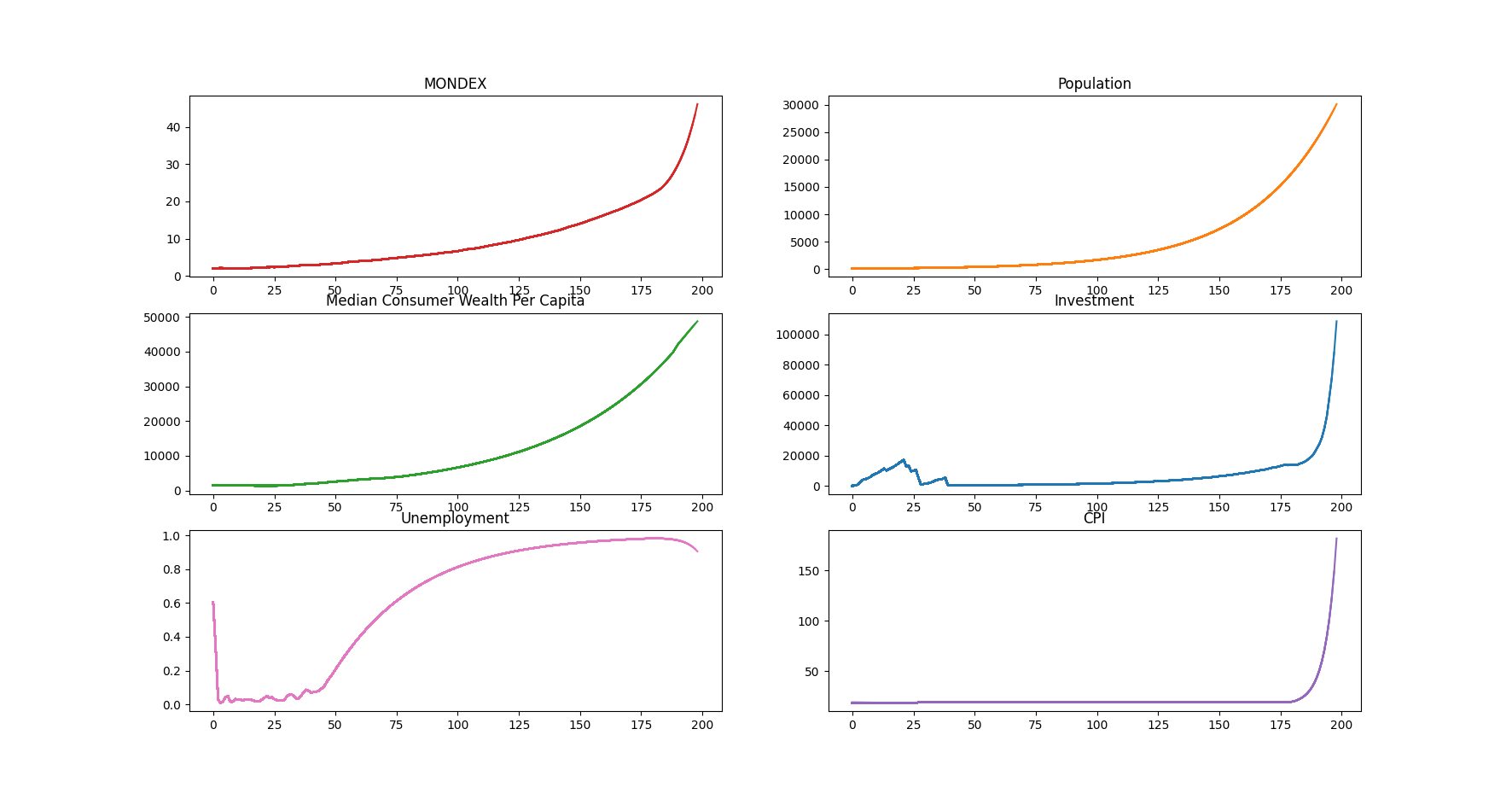
Some Interesting Charts
After running the simulation with the initial market conditions described above, here are some interesting graphs I created. A few things to note: I started the simulation with 100 agents, and the initial spike in unemployment (around turns 1-3) was driven by the lag it took for the majority of agents to move past the early squares and find jobs. Also, the simulation ended after 239 turns because all the agents had gone bankrupt.
I’d be interested in hearing your thoughts on what happened in this simulation, and I’ll discuss my own theory in a future post.